After reading it (it was great), I wanted to test my understanding of the paper by tallying up all experiments conducted within, calculating the total compute cost it would take to replicate the paper.
Headline result
Subset
Sources of uncertainty
FLOPs
Costs @ $3/H100/hr
Alignment
N/A
3.7e20
$888
LR variants (+default)
LR-sweeps, bayes search
7.99e23
$1.90M
LR variants (+optimal)
LR-sweeps
1.35e24
$3.22M
Epslion (Heatmaps)
LR-sweeps, $D$
1.34e24
$3.19M
Epslion (Full Sweeps)
LR-sweeps
7.99e23
$1.90M
Weight Decay
LR-sweeps
1.33e23
$317K
Adafactor vs Adam+PS
LR-sweeps, $D$
7.92e22
$188.5K
Compute Optimals
LR-sweeps, $D$
7.52e23
$1.79M
Total
too much
5.42e24
$12.9M
Any corrections on the numbers here will be appreciated.
Although I have made significant efforts to vet these claims, if I have made significant mistakes in mathematics, these results could be off by magnitudes.
Sidenote: What's an H100 worth?
Although it’s never stated, all experiments in the paper were almost certainly conducted with TPUs (because it’s from Google Deepmind). Furthermore, as there is no mention of int8 usage in their paper, it is most likely that all experiments were conducted with bfloat16 compute precision, per the nanodo default.
However, as a GPU user, I prefer to calculate compute in terms of H100 hours. Some basic facts:
The H100-SXM is reported as having 989.40TFLOP/s of 16-bit tensor core operations.
Also, 66.9TFLOP/s fp32 non-tensor, but I won’t consider non-tensor operations (such as softmax or hadamard products) in my analysis.
Recent pytorch blogs and torchtitan both report single-node FSDP’d bf16 H100 MFU for reasonably mid sized models at (optimistically) 40%.
the smaller models ($D<1024$) in the paper are unlikely to have MFU that high.
Although this is not hard to push higher with some manual tuning, the time spent tuning performance & engineering required to heuristically adjust for efficiency depending on setting is unlikely to be worth it.
The cost of a H100 node (at the time of writing) is $3.5/hr/gpu on lambdalabs, $2.85/hr/gpu from sfcompute, and ballpark $2/hr/gpu if you get a long term bulk contract.
If we pessimistically estimate the true average tensor FLOP/s provided by a H100 GPU on an average run as 3.5e14 (aka slightly above 35% MFU), and the cost of a H100 GPU as $3/hr, we get:
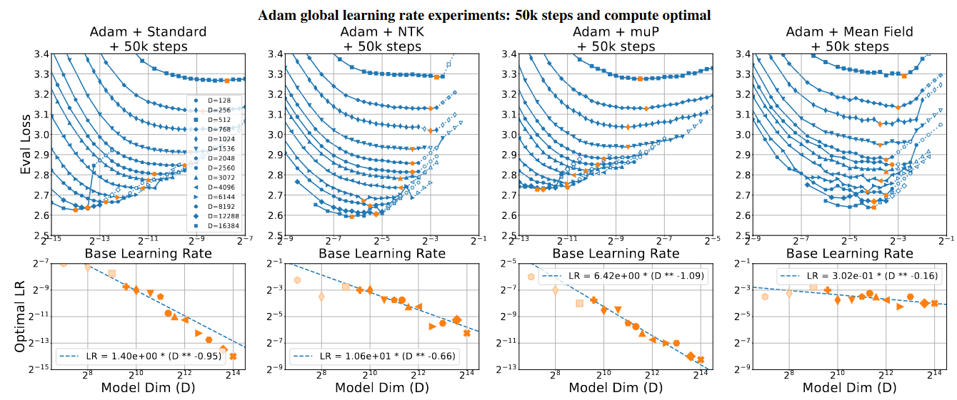
the 50k fixed step experiments are not the same as any of the above; they use “default constant learning rate multipliers” and have different power laws.
3x optim (SGD+moment, adam, adafactor)
4x parameterizations
LR experiment-like sweep across model width && LR.
width only goes up to 11x, last 3 are missing on Compute Optimal.
compute-optimal experiments use 20x tokens of non-embedding P as a heuristic.
However, there are many problems with the experimental summary as given above.
Problems
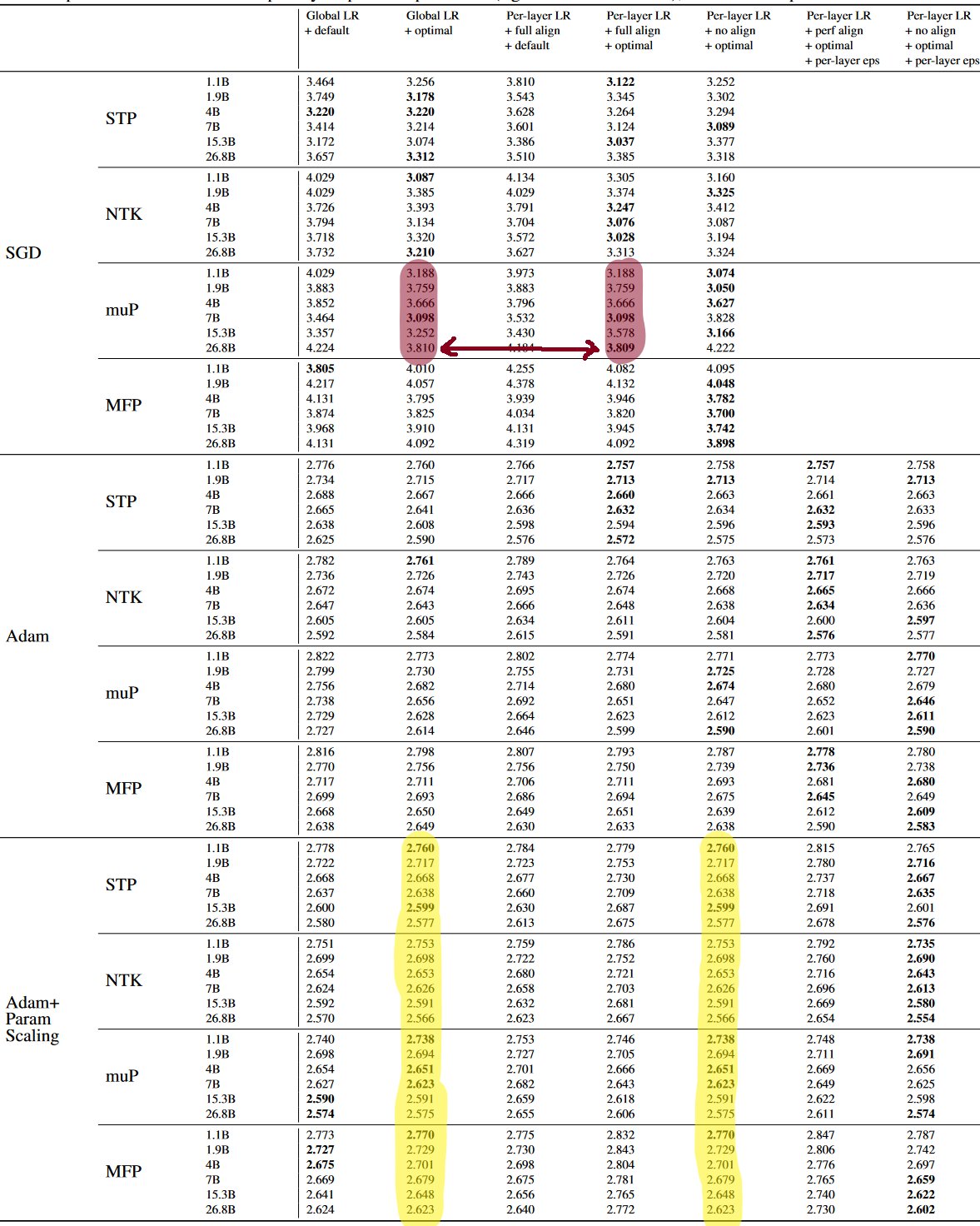
It is not clear whether they re-executed the per-layerLR experiments for the two edge cases where per-layer constants lead to identical behavior to globalLR (where $c_1 = c_l = c_{L+1}$):
muP + SGD + full alignment, or
Adafactor + any parameterization + no alignment
My expectation is that their experiments were repeated, because if you look at Table E1, you’ll see that the muP+SGD+full columns actually have a single diverging value (presumably caused by precision differences):
However, I was also given (private) notice that in some cases, the experiments with theoretically equivalent settings were merely executed once, with the eval losses copied twice. This makes the true extent of compute unknowable from the paper.
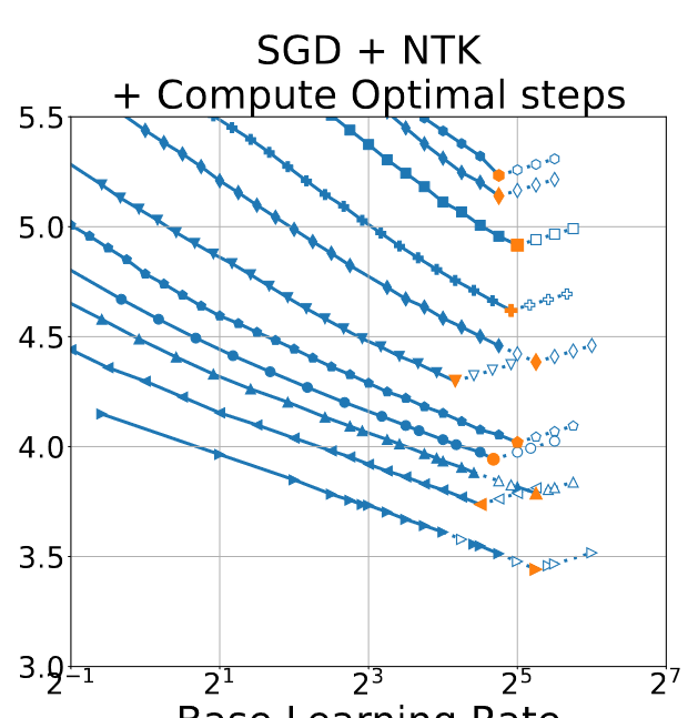
The LR experiments have indeterminate bounds, so I can’t directly figure out how many experiments were executed.
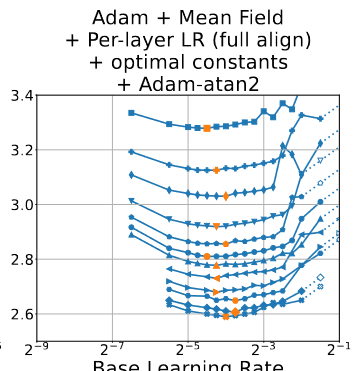
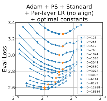
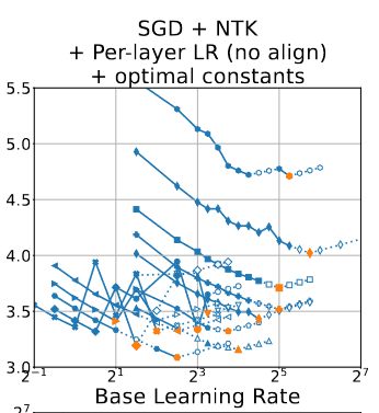
You can’t “just read the graphs” to figure out what the range of LRs used are either; they cut off the y/x axis:
Frankly, it doesn’t even look like the steps here are guaranteed to be split in intervals of $2^{0.25}\text{ or }2^{0.5}$.
After further inspection, it looks an awful lot like the runs have arbitrary LR ranges even for the same $D$, optim, parameterization, and alignment. Or I just don’t understand the selection process (what are the unshaded shapes?).
When tuning the per-layer constant multiplicative factors defined in Section 4.2, we use vizier to perform 3D hparam search for $(γ_1, γ_h, γ_{L+1})$ at $b = 1024$. Recall that we define the learning rate in layer $l$ as $η_l = β_n·γ_l·\frac{n}{b}^{−cl}$ and sweep one dimension at all model sizes to determine $β_n$, so these values of $(γ_1, γ_h, γ_{L+1})$ define two ratios where any common factor can be absorbed by $β_n$.
To be clear, that last segment means: “you can divide $(γ_1, γ_h, γ_{L+1})$ by any of the 3 values to obtain some $(\gamma_x, \gamma_y, 1)$ tuple, the sweep will bring $\beta_n$ back to the correct value”. And so they say:
For each optimizer × parameterization, we run 800 trials with at most 100 trials in parallel with a range set to $[1\text{e−}2, 1e2]$ for each constant. If the optimal value for any of the constants is at or near the edge of the range after this first search, we extend the range of the sweep for that constant to 0.01 and 100x the optimal value found in the original sweep and repeat the same tuning procedure.
Upside: this gives 800 experiments as a lower bound for the $\gamma$ experiments.
Downside: We otherwise have no plotted information about the 3D experiments that were conducted. The actual plotted graphs just show final eval loss against base LR, under the assumption that the $b=1024$ base line on the Optimal Constants graphs actually hide the extra work done to sweep $\gamma$ values.
It is deeply unclear to me what is actually implemented for the fixed-step vs compute optimal runs. If we look at the 50k steps graph:
I have no idea what the differences are supposed to be here. However, in the interest of sticking with the paper’s behaviour, I attempt to include the compute used for these psuedo-repeated experiments.
For each of these issues, I do my best to pick an approximation that makes sense to me in the later sections.
Transformer information
In Appendix C, the model is described as:
decoder-only
no bias on weights (including layernorm, which only has learnable scale)
LPE, pre-LN, GeLU, no tied emb
T5 Sentencepiece 32k + 1BOS + 100extra, i.e. $V=32101$. This is never stated to be padded.
“Training inputs are sequence-packed, while evaluation inputs are padded”
$$R_{\text{ffn}} - \text{[ffn dim : outer dim] ratio, assuming no GLU}$$
$$R_{kv} - \text{[num k or v heads : num att heads] ratio}$$
$$l_{seq} - \text{assumed average sequence length}$$
For all experiments except the compute-optimal series in Appendix I, we also have a hardcoded number of $steps=50000$ and global $BS=256$, making the total number of tokens seen per experiment $TPE=6.5536\text{e}9$ by default.
Subproblem: Alignment experiments
I assume the alignment experiments got their optimal LRs from the later experiments, and didn’t do their own sweeps, so that would make the cost simply,
$$
\sum_{d\in {1024,2048,4096}} 4\times\text{tokens per experiment}\times M(d)
$$
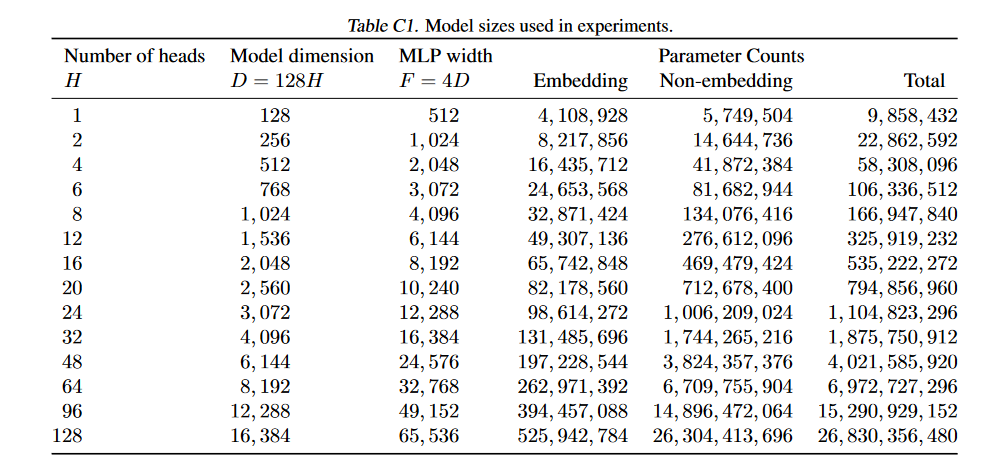
Table E1 has a neat collection of many of the runs done for obtaining the best eval losses under any given parameterization/optimizer/setting (some combination of global vs per-layer vs $\gamma$-optimal vs $\epsilon$-optimal).
This is an easier subproblem to tackle than the general issue of all LR sweeps, as the requirements are better known – though still not entirely determined, per the repetition ambiguity mentioned earlier. For that issue, I assume that all experiments were conducted, with no copied results, making the estimate here an upper bound.
We have the following schedule:
$D\in {3072, 4096, 6144, 8192, 12288, 16384}$
4x parameterizations
3x optimizers, where
SGD only receives 5 experimental settings
Adam & Adam+PS receives 7
$$
\sum_{d\in {3072,4096,6144,8192,12288,16384}} 4\times(5+7*2)\times\text{tokens per experiment}\times M(d)
$$
These would’ve taken slightly below $400k in H100 compute to execute. Reasonably speaking, this is within the bounds of SWE life savings / big academic budgets / TPU Research Cloud upper-class. Technically replicable, albeit not cheap.
But the bulk of the compute used in the paper comes from the LR sweeps, so we have to start working on that.
Estimating LR sweep damage
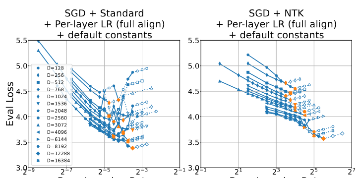
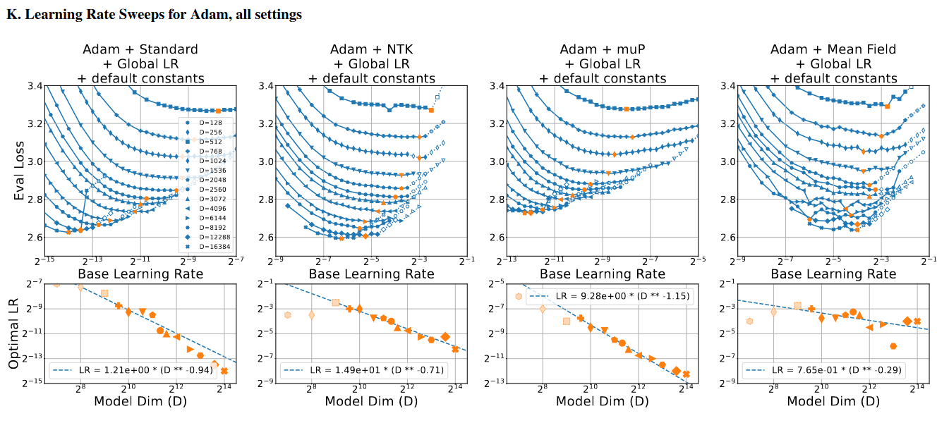
So, here’s a a graph:
Here’s another graph:
And here’s a third one:
Guess what?
There isn’t a constant num. of LRs sweeped for a given $D$, or optim/parameterization/setting.
Especially notable: number of runs seems inversely correlated with $D$; there are almost always less runs for the highest dim than the lowest.
Neither is there an observable cutoff for when the runs stop – runs will spike up to 2x the optimal no problem.
You can’t get the exact correct number of runs by graph-reading; in many cases the points are out-of-bounds.
The consistencies I do spot are that:
there is typically a “starting LR” (smallest base) for any given line.
the hollowed points are typically to the right – but sometimes left – of the optimal point.
so I think the mechanism worked this way:
start a sweep with a starting LR and some expected jumpsizes of $\sqrt{2}$ or $\sqrt{\surd 2}$.
terminate it by the 20% / NaN heuristic.
if the graph looks weird (optimal point somewhere odd), rerun to fill many $2^{0.25}$ intervals around the current optimal. These result in the plotted hollow points
I have no means of confirming this as the experimental procedure, as the authors of the paper stopped replying to me.
An arbitrary decision
Due to my desire to finish this blog post in a reasonable amount of time, I made the unprincipled decision of approximating the number of experiments-per-line in any given Eval Loss vs Base Learning Rate graph as 15.
Why 15? By eyeballing, the range of runs-per-line for the highest $D=16384$ hovers around 10~15. Although the lines with smaller D tend to have far more points on average, the amount of compute spent per run scales by $O(D^2)$, so I think this is fair enough.
Feel free to suggest a more principled approach if you have one.
Main problem: Epslion
Much of the compute used up by the paper comes from Section 4.3, the Adam epslion experiments.
Optimal eps runs
Now that we have an estimate of LRs-per-line as 15, we can estimate the compute spent on the actual Adam epslion varying graphs:
$$
\sum_{d} 4*(2+4) \times \text{points per line}\times\text{tokens per experiment}\times M(d)
$$
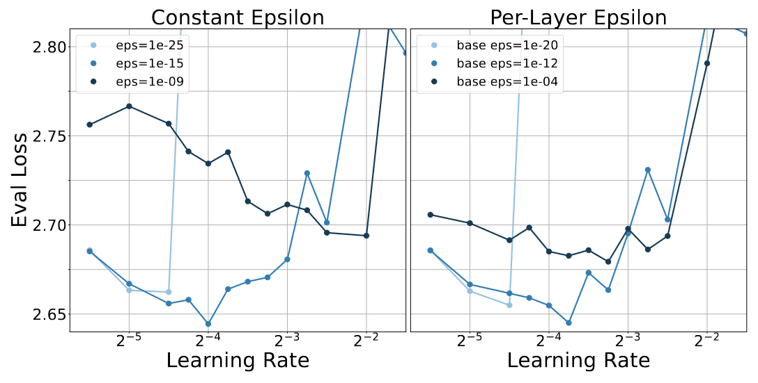
There are two ways you could approach the expected sweep range for this problem:
assume the LR experiment sweep code was reused. All 14x $D$, LR swept by arcane unknown ruleset.
Limit to the graphs. Only the last 6 values of $D$ were shown – assume only those were used. Plus, if we look at Figure 6:Notice that the range of evaluated learning rates actually seems constant here, unlike in the normal Eval Loss vs Base LR plots.
I’m picking the latter because it’s simpler. Would be happy to be shown evidence that this is wrong.
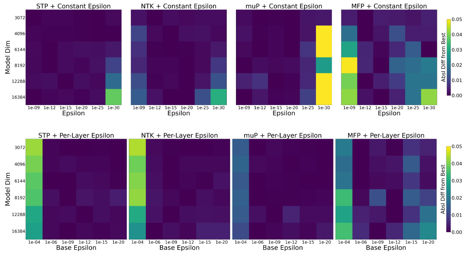
defeps_heatmaps()->int:# eps-type * eps-val * parameterizations * LR range * ...return2*6*4*13*TPE*sum(M(d)fordinD[-6:])'''
>>> f'{eps_heatmaps():.3E}';cost_of_run(eps_heatmaps())
'1.341E+24'
(3193533.466348094, 133063.89443117057)
'''
These squares are worth US$3.2 Million
To be clear, this is supposed to be an underestimate of the budget required, because we model the average number of unique LRs used per heatmap square as a constant $13$ instead of the (typically higher) value used in variable LR sweeps.
Main problem: LR Sweep Strategies
The other meat of the paper is in Section 4.2, the $\text{optimizer}\times\text{parameterization}\times D\times\text{LR setting}\times\text{alignment}\times\text{LR Sweeps}$ experiments.
$\beta$-only experiments
“$\beta$” refers to the empirically obtained base LR constant under the equation $\eta_l = \beta_n\cdot\frac{n}{b}^{-c_l}$, also known as the +default experiments.
The paper sweeps this for 3x optimizers, 4x parameterizations, 14x widths, global vs per-layer $c_l$, and of course unknown LR sweep counts.
$$ \sum_{d} 3*4*2 \times \text{points per line}\times\text{tokens per experiment}\times M(d) $$
Incidentally, this has an identical estimated cost to the epslion variants.
$\gamma$ experiments
So, two issues.
These experiments are “like” the $\beta$-only experiments, but with 3x cases (GlobalLR, Perlayer-fullalign, Perlayer-nolign) instead of 2x (GlobalLR, Perlayer-fullalign).
$$ \sum_{d} 3*4*3 \times \text{points per line}\times\text{tokens per experiment}\times M(d) $$
Specifically for $d=1024=b$, we have at least 800 extra runs, due to the 3D hparam search for $(\gamma_1, \gamma_h, \gamma_{L+1})$.
$$ 3*4*3*800 \times\text{tokens per experiment}\times M(1024) $$
We can combine those two as,
$$ 36\times\text{tokens per experiment}(800*M(1024) + \text{points per line}\sum_{d}\times M(d)) $$
The compute optimal experiments include models up to $H = 32$ or $H = 48$, and the fixed (50,000) step experiments include models up to $H = 128$.
If you read the graphs in Appendix I, this is slightly wrong, because
50k experiments go to $H=48$ on Adafactor, and $H=128$ otherwise
all compute optimal experiments go up to $H=32$ only.
Note that a 4B param run requires 80B tokens by chinchilla, and C4 is less than 200B tokens, so they couldn’t have gone higher without changing the dataset.
This is honestly a bit complex, so let’s forgo the latex and just describe it in python:
In the grand scheme of things, 5.42e24 is “not that big”. After all, that’s not even 15% of the compute used for Llama 3; a 100k H100 cluster could accomplish all of these experiments in just 2 days.